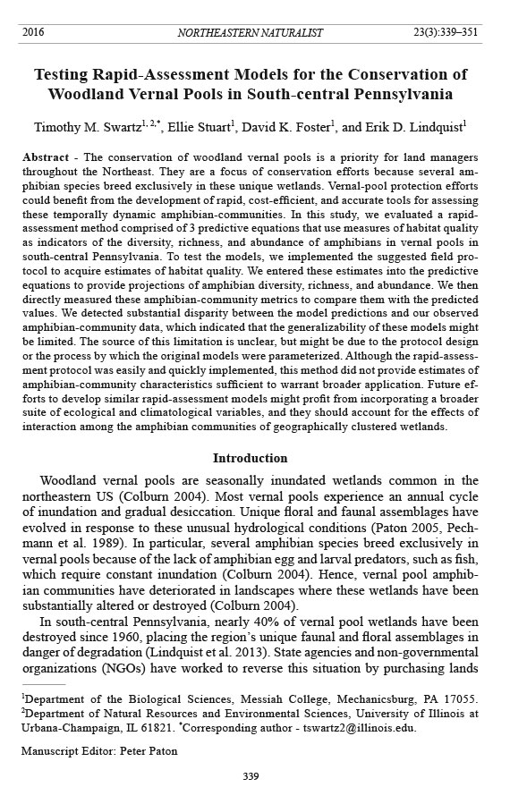
Northeastern Naturalist Vol. 23, No. 3 T.M. Swartz, E. Stuart, D.K. Foster, and E.D. Lindquist 2016 339 2016 NORTHEASTERN NATURALIST 23(3):339–351 Testing Rapid-Assessment Models for the Conservation of Woodland Vernal Pools in South-central Pennsylvania Timothy M. Swartz1, 2,*, Ellie Stuart1, David K. Foster1, and Erik D. Lindquist1 Abstract - The conservation of woodland vernal pools is a priority for land managers throughout the Northeast. They are a focus of conservation efforts because several amphibian species breed exclusively in these unique wetlands. Vernal-pool protection efforts could benefit from the development of rapid, cost-efficient, and accurate tools for assessing these temporally dynamic amphibian-communities. In this study, we evaluated a rapidassessment method comprised of 3 predictive equations that use measures of habitat quality as indicators of the diversity, richness, and abundance of amphibians in vernal pools in south-central Pennsylvania. To test the models, we implemented the suggested field protocol to acquire estimates of habitat quality. We entered these estimates into the predictive equations to provide projections of amphibian diversity, richness, and abundance. We then directly measured these amphibian-community metrics to compare them with the predicted values. We detected substantial disparity between the model predictions and our observed amphibian-community data, which indicated that the generalizability of these models might be limited. The source of this limitation is unclear, but might be due to the protocol design or the process by which the original models were parameterized. Although the rapid-assessment protocol was easily and quickly implemented, this method did not provide estimates of amphibian-community characteristics sufficient to warrant broader application. Future efforts to develop similar rapid-assessment models might profit from incorporating a broader suite of ecological and climatological variables, and they should account for the effects of interaction among the amphibian communities of geographically clustered wetlands. Introduction Woodland vernal pools are seasonally inundated wetlands common in the northeastern US (Colburn 2004). Most vernal pools experience an annual cycle of inundation and gradual desiccation. Unique floral and faunal assemblages have evolved in response to these unusual hydrological conditions (Paton 2005, Pechmann et al. 1989). In particular, several amphibian species breed exclusively in vernal pools because of the lack of amphibian egg and larval predators, such as fish, which require constant inundation (Colburn 2004). Hence, vernal pool amphibian communities have deteriorated in landscapes where these wetlands have been substantially altered or destroyed (Colburn 2004). In south-central Pennsylvania, nearly 40% of vernal pool wetlands have been destroyed since 1960, placing the region’s unique faunal and floral assemblages in danger of degradation (Lindquist et al. 2013). State agencies and non-governmental organizations (NGOs) have worked to reverse this situation by purchasing lands 1Department of the Biological Sciences, Messiah College, Mechanicsburg, PA 17055. 2Department of Natural Resources and Environmental Sciences, University of Illinois at Urbana-Champaign, IL 61821. *Corresponding author - tswartz2@illinois.edu. Manuscript Editor: Peter Paton Northeastern Naturalist 340 T.M. Swartz, E. Stuart, D.K. Foster, and E.D. Lindquist 2016 Vol. 23, No. 3 with vernal pools and working with landowners to lessen the impact of forestry and other activities on vernal pools (PNHP 2016). Due to limited funding, landconservation efforts generally prioritize potential land purchases according to the conservation value of parcels (Lindquist et al. 2013). Time-intensive survey methods such as pitfall trapping provide the most robust estimates of amphibian occupancy and community composition for wetlands (Corn 1994); however, these efforts often require numerous site visits, and can rarely be undertaken for more than a few pools simultaneously. Wetland-assessment protocols are a widely used alternative to comprehensive surveys for evaluating wetland biotic integrity and overall conservation value (Fennessy et al. 2004), but they usually require direct assessment of amphibian communities (e.g., Ohio Wetland Assessment; Micacchion 2004). Direct assessment of vernal pools can be challenging because amphibian activity in these habitats is subject to sudden, seasonal fluctuations (Colburn 2004). For example, while obligate vernal-pool species in the Northeast reproduce during just a few rainy nights in late February and early April, Scaphiopus holbrookii (Harlan) (Eastern Spadefoot) may stage its explosive breeding events at nearly any time of year when precipitation and temperature conditions are met (Colburn 2004), and many facultative species arrive at these ponds throughout much of the spring and early summer (Calhoun and DeMaynadier 2007, Colburn 2004). The activity of vernal pool amphibians can be so erratic that effective direct-assessment methods often require substantial investment of personnel and time. The primary objective of Lindquist et al. (2013) was to develop a reliable method of indirectly assessing amphibian biodiversity based on local habitat variables that are less prone to temporal variation than the amphibian communities themselves. Drawing on the wealth of vernal pool literature (Burne and Griffin 2005a, b; Compton et al. 2007; Paton 2005; Paton and Crouch 2002), Lindquist et al. (2013) identified critical habitat features, which they then quantified through field surveys. Those authors subsequently related the habitat variables to amphibian biodiversity through regression modeling, yielding a set of predictive equations for amphibian species diversity (AD; Shannon-Wiener index, H'), species richness (AR), and abundance (AA; raw abundance). Lindquist et al. (2013) sought to provide a set of tools that land managers could use to establish the conservation priority of vernal pools based on any or all of these biodiversity metrics, without committing substantial financial and human resources to intensive, direct assessments. Here we describe our effort to evaluate the reliability of these predictive models and assess their potential to be employed to protect these complex wetlands. Study Site Description In south-central Pennsylvania, vernal pools are concentrated along the base of the western and northwestern slope of South Mountain, an area representing the northernmost extent of the Blue Ridge Mountains (Lindquist et al. 2013). These ephemeral wetlands have been identified as important conservation targets by state and non-profit agencies (Pennsylvania Natural Heritage Program 2015). We identified potential study sites from maps produced by the Pennsylvania Chapter of the Northeastern Naturalist Vol. 23, No. 3 T.M. Swartz, E. Stuart, D.K. Foster, and E.D. Lindquist 2016 341 Nature Conservancy in 2005 using USGS quadrangle maps of Cumberland, Adams, York, and Franklin counties. We ultimately selected 30 pools for our study (Fig. 1). We randomly chose pools located on public lands (Michaux State Forest, Caledonia State Park, and lands managed by The Nature Conservancy) or which were made available to us by private landowners. Most of the selected pools were roughly circular or oblong depressions that lacked aquatic vegetation and were situated under a semi-open to closed forest canopy. Some pools were located over 300 m from the closest neighboring wetland, while others were amongst a cluster of pools. In an effort to simulate the approach that would be taken by a land manager possessing no prior knowledge of the amphibian community of a vernal pool of interest, we did not consider pool size, apparent quality, or known amphibian presence during the selection process. Methods Rapid-assessment models Lindquist et al. (2013) conducted surveys to quantify a suite of potential botanical, chemical, and physical variables to parameterize models of AD, AR, Figure 1. Study sites (black circles) across 56 km of the northwestern base of South Mountain (gray polygon) in Cumberland and Franklin Counties of Pennsylvania. Due to overlap, not all of the original 30 study sites are separately discernable in the inset. Northeastern Naturalist 342 T.M. Swartz, E. Stuart, D.K. Foster, and E.D. Lindquist 2016 Vol. 23, No. 3 and AA. They surveyed amphibians and plants, measured pool area and volume, and conducted water-chemistry tests at 21 vernal pools between February 2005 and February 2007. Due to early drying of 5 pools, only 16 of the 21 were included in the modeling process. The predictive models were developed using multiple linear-regression (MLR) modeling with stepwise forward addition of variables (Table 1). The 3 equations that resulted from this effort were estimated to account for the majority of the variation in AD, AR, and AA observed at vernal pools in the South Mountain region (R2 ≥ 0.7; Lindquist et al. 2013). Vegetation surveys We tested the 3 amphibian biodiversity models by following the rapid-assessment protocol described by Lindquist et al. (2013) between May 2014 and May 2015. We conducted vegetation surveys between 27 May and 25 June 2014 following the prescribed methods (Lindquist et al. 2013). We divided the upland area within 50 m of the pool into 4 quadrants opening to the 4 cardinal directions. We surveyed the vegetation in each quadrant within 5 randomly placed 5 m x 5 m quadrats. We specified percent cover by herbaceous plant, fern, shrub, and tree species. For the analysis, we did not differentiate among trees by size class. We also visually estimated the overall percent cover of Sphagnum spp. (sphagnum mosses) within 2 m of the pool edge. In addition, Lindquist et al. (2013) excluded graminoids, a polyphyletic grouping that includes the families Cyperaceae (sedges), Poaceae (grasses), and Juncaceae (rushes), from the vegetative analysis in their models because their inclusion would have inhibited a rapid assessment due to the difficulty of this group’s taxonomic identification. Pool surveys In June 2014, we surveyed pond perimeters with a Trimble GeoXT GPS receiver (Trimble, Sunnyvale, CA) and calculated pool area (m2) using GPS Pathfinder Office on-board software (v. 4.00, Trimble, Sunnyvale, CA). We conducted waterchemistry tests and estimated pool volume in April 2015. We used a HACH DR/850 colorimeter (HACH Company, Loveland, CO) to conduct measurements of FAU turbidity and dissolved phosphates (PO4 mg/L). We calculated pool volume (m3) by multiplying pool area by the mean of water-depth measurements collected at 1-m intervals along 2 perpendicular transects of the pool. Eight of our pools had not filled as of our sampling date; thus, we included only the 22 inundated pools in our analyses. Amphibian surveys We followed the methods from Lindquist et al. (2013) to conduct amphibian quadrat surveys during a 2-week period between 26 June and 10 July 2014, similar to the timeframe used by Lindquist et al. (2013). At this point in the summer, many pools had begun to desiccate or were already dry, forcing amphibians to take refuge in the nearby uplands, which we surveyed through the quadrat surveys. We randomly placed one 5 m x 5 m quadrat in each cardinal direction quadrant. Within each quadrat, we rolled and replaced logs and raked and replaced ground leaf-litter. We Northeastern Naturalist Vol. 23, No. 3 T.M. Swartz, E. Stuart, D.K. Foster, and E.D. Lindquist 2016 343 Table 2. Descriptive statistics and differences between pond parameters from this study and Lindquist et al. (2013) based on Mann-Whitney U tests (df = 40 for pool volume and 41 for all other parameters). See Table 1 for parameter abbreviations. *Denotes results significant at the 0.001 level; **Denotes results significant at the less than 0.001 level. Mean SD Minimum Maximum Parameter This study Lindquist This study Lindquist This study Lindquist This study Lindquist U Z P HSR 11.04 16.81 9.33 6.45 3.00 6.00 35.00 31.00 91.5 2.4927* 0.0063 HSD 1.51 1.71 0.60 0.27 0.35 1.04 2.79 2.39 139 1.0791 0.1403 SSD 1.46 1.53 0.32 0.36 1.04 0.99 2.18 2.39 154 0.6357 0.2625 TSD 2.87 1.86 1.15 0.25 1.45 1.32 5.29 2.19 78 2.8827* 0.0020 TCC 121.1 211.59 22.28 133.78 85.50 125.60 161.95 697.60 22 4.5383** less than 0.001 CWD 2.37 0.74 1.77 0.37 0.70 0.21 8.00 1.40 31.5 4.2577** less than 0.001 Area (m2) 659.56 456.44 962.65 421.66 128.99 50.00 4744.80 1409.00 144 0.9313 0.1758 Volume (m3) 212.14 177.31 209.04 167.01 23.12 15.50 923.20 475.30 149 0.7835 0.2167 Turbidity 32.81 80.00 30.70 60.15 1.00 26.00 140.00 239.00 49.5 3.7271** less than 0.001 PO4 0.93 2.53 1.04 0.45 0.00 1.35 2.75 2.75 40.5 4.0950** less than 0.001 Table 1. The Lindquist et al. (2013) multiple linear regression models for predicting values for amphibian species diversity, amphibian species richness, and amphibian abundance. The independent variables are listed in the order in which they were added to the models through stepwise analysis. HSR = herb and fern species richness, TCC = tree canopy cover, PS = percent perimeter sphagnum, HSD = herb and fern species diversity, SSD = shrub species diversity, TSD = tree species diversity, and CWD = coarse woody debris. Model Intercept Var 1 (coeff.) Var 2 (coeff.) Var 3 (coeff) Var 4 (coeff.) Var 5 (coeff.) Diversity -0.857 HSR (0.055) TCC (0.001) PO4 (0.397) PS (-0.236) - Richness -1.739 HSR (0.161) Turbidity (-0.007) PO4 (1.22) Volume (0.005) PS (-0.773) Abundance -61.430 HSD (12.865) SSD (7.814) TSD (11.948) Area (0.01172) CWD (2.964) Northeastern Naturalist 344 T.M. Swartz, E. Stuart, D.K. Foster, and E.D. Lindquist 2016 Vol. 23, No. 3 calculated AA and AD from this quadrat-survey data. We also conducted visual encounter surveys (VES; Guzy et al. 2014) at each site once in either June or July 2014 (30 min) and once in April 2015 (60 min). We conducted pool surveys (presence–absence) in April 2015 by identifying egg masses and adult individuals in the ponds. We calculated amphibian species richness using the Lindquist et al. (2013) survey protocol and included the combined results of the quadrat, in-pool, and perimeter surveys. We excluded in-pool data from AD and AA calculations for 2 reasons: (1) larval counts would have been difficult to standardize, and (2) adult counts are difficult to accurately assess without the use of time-consuming pitfall traps. Model validation We used the AD, AR, and AA models to provide predictions for the amphibian biodiversity metrics for our 22 vernal pools by substituting our observed values for percent canopy cover; herbaceous plant, shrub, and tree richness and diversity; pool area and volume; and water chemistry for the corresponding variables in the Lindquist et al. (2013) models (Table 1). To evaluate the models’ predictive accuracies we compared our observed values for AR, AD, and AA to those predicted by the models. Following Piñeiro et al. (2008), we concluded that there was correspondence between the predicted and observed values if: (1) there was a statistically significant linear relationship between the observed and predicted values, and (2) that relationship was described by a linear-trend line with a slope not significantly different from one. To establish these criteria, we conducted a regression of the predicted values (x-axis) on the observed values (y-axis) and calculated the P- and R2-values for a fitted linear-trend line. We then compared the trend-line slope with that of a reference line passing through the origin (slope = 1; Cohen and Cyert 1961, Piñeiro et al. 2008, Power 1993) using the SlopesTest array function in the Real Statistics Resource Pack software (Release 4.3; www.real-statistics.com) developed for Microsoft Excel 2013 (Microsoft Corporation, Redmond, WA). To investigate the source of any potential lack of correspondence, we conducted Mann-Whitney U tests (Mann and Whitney 1947) to determine whether the measurements for the botanical, chemical, and physical parameters differed significantly between our sample and Lindquist et al.’s (2013) sample. These tests were conducted using the Non-parametric Tests tool in the Real Statistics Resource Pack software. We set α = 0.05 for all statistical tests. Results There was no significant relationship between observed values and predicted values for AD (P = 0.7684), AR (P = 0.6033), and AA (P = 0.5210), and the slope of the linear-trend lines for all 3 metrics differed significantly from a reference line (slope = 1; Fig. 2). Not only did linear regression show considerable disparity between observed and predicted values for all 3 metrics, but many predictions were biologically unrealistic (i.e., a negative prediction for a quantity that is theoretically positive). For AD (Fig. 2A), 13 of the 22 predictions were negative values (59.1%), for AR, 10 of the predictions were negative values (45.5%), and a total of 13 pools Northeastern Naturalist Vol. 23, No. 3 T.M. Swartz, E. Stuart, D.K. Foster, and E.D. Lindquist 2016 345 Figure 2. Regression plots. Full caption provided on the following page. Northeastern Naturalist 346 T.M. Swartz, E. Stuart, D.K. Foster, and E.D. Lindquist 2016 Vol. 23, No. 3 were predicted to have an AR value of ≤1 (Fig. 2B). Of these 13 pools, 7 had supported the greatest observed amphibian richness of all the pools in our study. For AA, 6 of the 22 predictions were negative (27.3%), and of the 7 pools for which we observed no amphibians, the prediction was zero or less for only 3 (Fig. 2C). Botanical, physical, and chemical parameters exhibited substantial variation across study sites. In addition, Mann-Whitney U tests demonstrated that there was a significant difference between our data and those of Lindquist et al. (2013) for herbaceous species richness (HSR), tree species diversity (TSD), total percent canopy- cover (TCC), FAU turbidity, and dissolved phosphates (PO4), but no significant difference for shrub-species diversity (SSD), herbaceous plant-species diversity (HSD), pool area, or pool volume (Table 2). We encountered 3–6 amphibian species (mean = 4.68 ± 1.29) using a combination of VES, quadrat sampling, and pool surveys (Table 3). As expected, AD and AA measurements yielded fewer amphibians because they were limited to quadrat surveys. We encountered only 1 amphibian species at 6 pools and 0 species at 7 pools. The observed Shannon-Wiener diversity-index value (H') for these 13 pools was zero. In our study, quadrat surveys yielded fewer species than Lindquist et al. (2013) reported for this method (8 species vs. 13 species; Table 3). Riparian salamanders (Eurycea spp.) and Lithobates catesbeianus (American Bullfrog) were absent from our study sites, but Plethodon cinereus (Northern Redback Salamander) frequency was similar in both studies. Lithobates sylvaticus (Wood Frog) occurred at a greater frequency at the Lindquist et al. (2013) study sites, though we encountered Ambystoma opacum (Marbled Salamander) at a greater proportion of our pools. We documented a total of 13 amphibian species from the combined results of the VES, in-pool surveys, incidental encounters, and quadrat surveys. Ten of the species encountered were common to both studies, and the frequencies of occurrence did not differ significantly (P = 0.0956). However, we did find that a combination of VES, pool, and quadrat surveys yielded significantly higher species-richness values than our quadrat surveys alone (P < 0.001). Discussion Our intention in this study was to establish the level of predictive accuracy, biological relevance, and generalizability of these rapid-assessment models. Therefore, we considered the Lindquist et al. (2013) rapid-assessment models in terms Figure 2 (previous page). Plots of the regression of observed on predicted values for (A) amphibian species diversity, (B) amphibian species richness, and (C) amphibian abundance. Actual values for amphibian species diversity and amphibian abundance were calculated from quadrat surveys. Amphibian species richness was calculated from the sum of quadrat survey, VES, and pool-survey results. The equation and R2-value of the fitted linear-trend line (dashed line) is provided for each comparison. Not only do the low R2-values indicate that there was only a very weak relationship between the predicted and observed values, but the slopes of the fitted trend-lines for amphibian species diversity, amphibian species richness, and amphibian abundance all differ significantly from that of the reference line (P < 0.0001). Northeastern Naturalist Vol. 23, No. 3 T.M. Swartz, E. Stuart, D.K. Foster, and E.D. Lindquist 2016 347 of the mathematical correspondence between the predictions and observations, the degree to which the predictions were biologically realistic, and the potential for land managers to successfully use these models to focus conservation efforts on wetlands of high conservation value. In terms of mathematical accuracy, we have noted that the observed values for the 3 amphibian biodiversity metrics diverged from the models’ predictions, and that many of those predictions were biologically unrealistic. These observations provided an initial indication that the models may have been inappropriately estimated (Snee 1977). We confirmed this possibility when we temporarily ignored the precise numerical values and used the models’ predictions to rank the study pools according to their predicted conservation value. Using this protocol, we successfully identified ≤2 of the 5 pools (≤40%) that we observed to host the greatest AD, AR, and AA. When considered together, these observations compelled us to conclude that the generalizability of the rapid-assessment models is limited. We have identified several potential explanations for these results, though our data do not allow us to conclude which possibility accounts for our findings. The failure of the predictions to accurately characterize the amphibian communities as described by the observational data we gathered could be based in any of the following aspects of the modeling and verification processes: (1) the model-parameterization process, (2) the sample size used to parameterize the predictive models, Table 3. Frequency values for amphibians encountered at 22 pools during our amphibian surveys, and from Lindquist et al. (2013). We report the species encountered during quadrat surveys (Q), from terrestrial visual encounter surveys (VES), and from pool surveys (P). Nomenclature follows Collins and Taggart (2009). *indicates obligate vernal pool species. Frequency Lindquist Present study et al. (Q+VES Species (Q) (Q) +P) Ambystoma jeffersonianum (Green) (Jefferson Salamander)* - 0.05 0.14 Ambystoma maculatum (Shaw) (Spotted Salamander)* 0.14 0.05 0.82 Ambystoma opacum (Gravenhorst) (Marbled Salamander)* 0.05 0.18 0.36 Anaxyrus americanus (Holbrook) (American Toad) 0.43 0.18 0.36 Eurycea bislineata (Green) (Northern Two-lined Salamander) 0.10 - - Eurycea longicauda longicauda (Green) (Eastern Long-tailed Salamander) 0.10 - - Hemidactylium scutatum (Temminck & Schlegel) (Four-toed Salamander) 0.10 - 0.05 Lithobates catesbeianus (Shaw) (American Bullfrog) 0.10 - - Lithobates clamitans melanotus (Rafinesque) (Green Frog) 0.19 - 0.32 Lithobates palustris (LeConte) (Pickerel Frog) - - 0.05 Lithobates sylvaticus (LeConte) (Wood Frog)* 0.76 0.36 0.91 Notopthalmus viridescens (Rafinesque) (Eastern Newt) 0.10 - 0.23 Plethodon cinereus (Green) (Northern Redback Salamander) 0.38 0.41 0.95 Plethodon glutinosus (Green) (Northern Slimy Salamander) 0.14 0.05 0.27 Pseudacris crucifer (Wied-Neuwied) (Spring Peeper) 0.10 0.05 0.59 Scaphiopus holbrookii (Harlan) (Eastern Spadefoot)* - - 0.05 Mean Richness 2.86 1.32 4.68 SD 1.31 1.21 1.29 Northeastern Naturalist 348 T.M. Swartz, E. Stuart, D.K. Foster, and E.D. Lindquist 2016 Vol. 23, No. 3 (3) the methods by which amphibian-community data were collected, and (4) the specific predictor variables selected and sampled by Lindquist e t al. (2013). MLR modeling and step-wise regression procedures pose some historic challenges to ecological modeling. The R2 values reported by Lindquist et al. (2013) for the AD, AR, and AA models were high—0.7275, 0.8294, and 0.8823, respectively. However, in MLR modeling, R2 values may belie the true limits of a model’s generalizability. Step-wise regression modeling is prone to emphasizing chance variation within a data set and providing inflated R2 values (Hurvich and Tsai 1990; Kline 2011). Hence, we cannot rule out that the MLR modeling conducted by Lindquist et al. (2013) is a primary cause of the inaccurate predictions provided by the models. The patterns identified through ecological studies depend on the size and representativeness of the sample (Cao et al. 2002). The inaccurate predictions provided by the Lindquist et al. (2013) models may also be the result of the sample size used to parameterize these models (n = 16). Indeed, for several botanical and chemical parameters, Mann-Whitney U tests showed significant differences between the characteristics of our study sites and those studied by Lindquist et al. (2013). Some of our more puzzling results may have arisen from this limitation. For example, the MLR modeling process for AD and AR assigned relatively large, negative coefficients to percent perimeter sphagnum-coverage (PS; -0.236 and -0.773, respectively; Table 1). Neither the results of the present study nor the body of vernal pool literature support this strong inverse relationship (but see Hagstrom 1981 and Saber and Dunson 1978). Although achieving a large sample size is time-intensive, and ecosystem-scale studies are challenging, woodland vernal pools and their biotic communities may be too variable to be sufficiently characterized by smaller samples. Interestingly, we did not observe significant differences in pool size (area and volume) between the 2 sets of pools. Pool size has a well-known relationship to hydroperiod, which plays a primary role in structuring and regulating vernal pool communities (Colburn 2004, Pechmann et al. 1989, Snodgrass et al. 2000). Had we observed a significant difference in pool-size parameter measurements between the 2 studies, we could have concluded that it was a primary cause of the disparity between our predicted and observed results. As noted, rapid assessment of vernal-pool amphibian communities can be challenging because their abundance and activity varies substantially by weather and season (Colburn 2004). Hence, in addition to factors directly related to the modeling process, the inaccurate model predictions may have been due to the amphibian survey protocol. As demonstrated through comparison of our quadrat-only results and combined VES, quadrat, and in-pool survey results, sampling effort and method can have significant impacts on the amphibian-biodiversity estimates. We recommend that future efforts to develop rapid-assessment models of woodland vernal pools should rely on amphibian biodiversity estimates acquired from a more intensive survey, and hence, a not-so-rapid methodology. Furthermore, we recommend that spatially explicit, landscape-scale variables be incorporated into future efforts to model vernal pools. There were marked Northeastern Naturalist Vol. 23, No. 3 T.M. Swartz, E. Stuart, D.K. Foster, and E.D. Lindquist 2016 349 differences between the amphibian assemblages sampled in the 2 studies. We believe much of this difference is attributable to landscape features which were not incorporated into these models. Lindquist et al. (2013) noted that the presence of 2 salamander species typical of riparian wetlands (Eurycea spp., Table 3) correlated with “four woodland vernal pools that occasionally received input from nearby [springs or] streams during flooding events”. In addition, 3 other pools were located near other semi-permanent or permanent wetlands and well within the dispersal range of amphibians dwelling there (E.D. Lindquist, pers. observ.). The proximity of such wetlands would explain the presence in the Lindquist et al. (2013) study of true frog species (Lithobates spp.) that are sometimes found in vernal pools during wetter years (Colburn 2004). Based on these observations, it can be inferred that the interaction between ephemeral pools and nearby permanent wetlands may not be insignificant. By incorporating landscape context into modeling efforts, future workers might be able to account for these effects. An approach that differentiates between categories of ephemeral wetlands (e.g., Schrank et al. 2015) could be useful in cases where complex amphibian communities emerge as a result of the landscape-scale interaction between ephemeral pools and semi-permanent/permanent wetlands. We also identified extenuating circumstances that may have affected our work. Disrupted precipitation patterns linked to El Niño events have been implicated in changes in amphibian-population stability (e.g., Alexander and Eischeid, 2002). During the Lindquist et al. (2013) study period, weak El Niño events were observed, with atypical ocean temperatures in the El Niño 3.4 region occurring between June 2004 through May 2005 and again between August 2006 and February 2007 (NOAA 2016). No such phenomena were observed during our study period (NOAA 2016). In addition, rainfall totals and the frequency of rainfall events totaling 2 cm or more were 13.5% and 12.5%, respectively, higher in the South Mountain region in 2006 than in 2014. The predictive models do not include climatic variables; thus, the effect of this variation on amphibian communities is left unaccounted for, potentially limiting the accuracy of these models when implemented under climatic conditions dissimilar to those of the original study. The complexity of vernal pools is a testament to the ecological value they add to Northeastern landscapes, but as we have shown, it also hinders efforts to develop tools to rapidly assess these unique wetlands. Based on our work, we believe that vernal pool communities could be better characterized through more-standard, non-rapid assessment methods, particularly those that are parameterized with moreintensive amphibian surveys that incorporate environmental factors and landscape features in addition to local habitat parameters. Acknowledgments We thank the Department of Biological Sciences and the School of Science, Engineering, and Health at Messiah College for providing institutional support for this research. Financial support was provided through the Steinbrecher Undergraduate Summer Research Program, made possible through the generosity of Dr. Leroy and Mrs. Eunice Northeastern Naturalist 350 T.M. Swartz, E. Stuart, D.K. Foster, and E.D. Lindquist 2016 Vol. 23, No. 3 Steinbrecher. We also thank the students of the Spring 2015 Herpetology course at Messiah College for assisting with field surveys. Finally, we are indebted to the landowners for granting us access to their properties and to Sam Wilcock and T.J. Benson for providing valuable input on analysis. Literature Cited Alexander, M.A., and J.K. Eischeid. 2002. Climate variability in regions of amphibian declines. Conservation Biology 15:930–942. Burne, M.R., and C.R. Griffin. 2005a. Habitat associations of pool-breeding amphibians in eastern Massachusetts, USA. Wetlands Ecology and Management 13:247–259. Burne, M.R., and C.R. Griffin. 2005b. Protecting vernal pools: A model from Massachusetts, USA. Wetlands Ecology and Management 13:367–375. Calhoun, A.J., and P.G. DeMaynadier. 2007. Science and Conservation of Vernal Pools in Northeastern North America. CRC Press, Boca Raton, FL. 392 pp. Cao, Y., D.D. Williams, and D.P. Larsen, 2002. Comparison of ecological communities: The problem of sample representativeness. Ecological Monographs 72:41–56. Cohen, K.J., and R.M. Cyert. 1961. Computer models in dynamic economics. Quarterly Journal of Economics 75:112–127. Colburn, E.A. 2004. Vernal Pools: Natural History and Conservation. MacDonald and Woodward Publishing Co., Blacksburg, VA. 426 pp. Collins, J.T., and T.W. Taggart. 2009. Standard Common and Scientific Names for North American Amphibians, Turtles, Reptiles, and Crocodilians. 6th Edition. The Center for North American Herpetology, Lawrence, KS. 44 pp. Compton, B.W., K. McGarigal, S.A. Cushman, and L.R. Gamble. 2007. A resistant-kernel model of connectivity for amphibians that breed in vernal pools. Conservation Biology 21:788–799. Corn, P.S. 1994. Straight-line drift fences and pitfall traps. Pp. 109–117, In W.R. Heyer, M.A. Donnelly, R.W. McDiarmid, L.-A. C. Hayek, and M.S. Foster (Eds.). Measuring and Monitoring Biological Diversity: Standard Methods for Amphibians. Smithsonian Institution Press, Washington, DC. 364 pp. Fennessy, M.S., A.D. Jacobs, and M.E. Kentula. 2004. Review of rapid methods for assessing wetland condition. EPA/620/R-04/009. US Environmental Protection Agency, Washington, DC. 82 pp. Guzy, J.C., S.J. Price, and M.E. Dorcas. 2014. Using multiple methods to assess detection probabilities of riparian-zone anurans: Implications for monitoring. Wildlife Research 41:243–257. Hagstrom, T. 1981. Reproductive strategy and success of amphibians in waters acidified by atmospheric pollution. Pp. 55–57, In J. Coborn (Ed.). Proceedings of the European Herpetological Symposium, Oxford. Cotswold Wild Life Park Limited Buford, UK. 137 pp. Hurvich, C.M., and C. Tsai. 1990. The impact of model selection on inference in linear regression. The American Statistician 44:214–217. Kline, R.B. 2011. Principles and Practice of Structural Equation Modeling. 3rd Edition. Guilford Press, New York, NY. 427 pp. Lindquist, E.D., D.K. Foster, S.P. Wilcock, and J.S. Erikson. 2013. Rapid-assessment tools for conserving woodland vernal pools in the northern Blue Ridge Mountains. Northeastern Naturalist 20:397–418. Northeastern Naturalist Vol. 23, No. 3 T.M. Swartz, E. Stuart, D.K. Foster, and E.D. Lindquist 2016 351 Mann, H.B., and D.R. Whitney. 1947. On a test of whether one of two random variables is stochastically larger than the other. Annals of Mathematical Statistics 18:50–60. Micacchion, M. 2004. Integrated wetland-assessment program. Part 7: Amphibian index of biotic integrity (AmphIBI) for Ohio wetlands. Ohio EPA Technical Report WET/2004-7. Ohio Environmental Protection Agency, Wetland Ecology Group, Division of Surface Water, Columbus, OH. National Oceanic and Atmospheric Association (NOAA). 2016. Climate Prediction Center. Monitoring and Data: ENSO Impacts on the US—Previous Events. Available online at http://www.cpc.ncep.noaa.gov/products/analysis_monitoring/ensostuff/ensoyears. shtml. Accessed 17 February 2016. Paton, P.W. 2005. A review of vertebrate-community composition in seasonal forest pools of the northeastern United States. Wetlands Ecology and Management 13:235–246. Paton, P.W., and W.B. Crouch. 2002. Using the phenology of pond-breeding amphibians to develop conservation strategies. Conservation Biology 16:194–204. Pechmann, J.H., D.E. Scott, J.W. Gibbons, and R.D. Semlitsch. 1989. Influence of wetland hydroperiod on diversity and abundance of metamorphosing juvenile amphibians. Wetlands Ecology and Management 1:3–11. Pennsylvania Natural Heritage Program (PNHP). 2016. Vernal Pools. Available online at http://www.naturalheritage.state.pa.us/VernalPools.aspx. Accessed 1 August 2016. Piñeiro, G., S. Perelman, J.P. Guerschman, and J.M. Paruelo. 2008. How to evaluate models: Observed vs. predicted or predicted vs. observed? Ecological Modelling 216:316–322. Power, M. 1993. The predictive validation of ecological and environmental models. Ecological Modelling 68:33–50. Saber, P.A., and W.A. Dunson. 1978. Toxicity of bog water to embryonic and larval anuran amphibians. Journal of Experimental Zoology 204:33–42. Schrank, A.J., S.C. Resh, W.J. Previant, and R.A. Chimner. 2015. Characterization and classification of vernal pool vegetation, soil, and amphibians of Pictured Rocks National Lakeshore. American Midland Naturalist 174:161–179. Snee, R.D. 1977. Validation of regression models: Methods and examples. Technometrics 19:415–428. Snodgrass, J.W., M.J. Komoroski, A.L. Bryan, and J. Burger. 2000. Relationships among isolated wetland size, hydroperiod, and amphibian-species richness: Implications for wetland regulations. Conservation Biology 14:414–419.