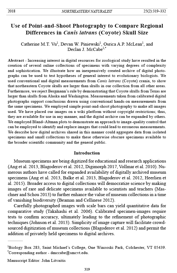
Use of Point-and-Shoot Photography to Compare Regional Differences in Canis latrans (Coyote) Skull Size
Catherine M.T. Vu, Devan W. Piniewski, Osrica A.P. McLean, and Declan J. McCabe
Northeastern Naturalist, Volume 25, Issue 2 (2018): 319–332
Full-text pdf (Accessible only to subscribers. To subscribe click here.)

Access Journal Content
Open access browsing of table of contents and abstract pages. Full text pdfs available for download for subscribers.
Current Issue: Vol. 30 (3)

Check out NENA's latest Monograph:
Monograph 22


Northeastern Naturalist Vol. 25, No. 2
C.M.T. Vu, D.W. Piniewski, O.A.P. McLean, and D.J. McCabe
2018
319
2018 NORTHEASTERN NATURALIST 25(2):319–332
Use of Point-and-Shoot Photography to Compare Regional
Differences in Canis latrans (Coyote) Skull Size
Catherine M.T. Vu1, Devan W. Piniewski1, Osrica A.P. McLean1, and
Declan J. McCabe1,*
Abstract - Increasing interest in digital resources for zoological study have resulted in the
creation of several online collections of specimens with varying degrees of complexity
and sophistication. We illustrate how an inexpensively created archive of digital photographs
can be used to test hypotheses of general interest to evolutionary biologists. We
used conventional and digital measurements from Canis latrans (Coyote) crania, to show
that northeastern Coyote skulls are larger than skulls in our collection from all other areas.
Furthermore, we reject Bergmann’s rule by demonstrating that Coyote skulls from Texas are
larger than skulls from Alaska and Washington. Measurements taken from calibrated digital
photographs support conclusions drawn using conventional hands-on measurements from
the same specimens. We employed simple point-and-shoot photography to make all images
used. We have placed our images on a wiki platform without copyright restrictions; thus,
they are available for use in any manner, and the digital archive can be expanded by others.
We employed Bland–Altman plots to demonstrate an approach to image-quality control that
can be employed to identify and replace images that could lead to erroneous measurements.
We describe how digital archives shared in this manner could aggregate data from isolated
specimens and small collections to make these otherwise obscure specimens available to
the broader scientific community and the general public.
Introduction
Museum specimens are being digitized for educational and research applications
(Ang et al. 2013, Blagoderov et al. 2012, Digimorph 2017, Vollmar et al. 2010). Numerous
authors have called for expanded availability of digitally archived museum
specimens (Ang et al. 2013, Balke et al. 2013, Blagoderov et al. 2012, Heerlien et
al. 2015). Broader access to digital collections will democratize science by making
images of rare and delicate specimens available to scientists and teachers (Maschner
and Schou 2013) to further enhance the value of museum collections in a time
of vanishing biodiversity (Beaman and Cellinese 2012).
Carefully photographed images with scale bars can yield quantitative data for
comparative study (Takahashi et al. 2006). Calibrated specimen-images require
tests to confirm accuracy, ultimately leading to the refinement of photographic
techniques (Johnson et al. 2013). Simplicity of image capture will facilitate crowdsourced
digitization of museum collections (Blagoderov et al. 2012) and permit the
addition of privately held specimens to digital archives.
1Biology Box 283, Saint Michael’s College, One Winooski Park, Colchester, VT 05439.
*Corresponding author - dmccabe@smcvt.edu.
Manuscript Editor: John Litvaitis
Northeastern Naturalist
320
C.M.T. Vu, D.W. Piniewski, O.A.P. McLean, and D.J. McCabe
2018 Vol. 25, No. 2
Saint Michael's College (Colchester, VT) students assembled a digital museum
collection of C. latrans Say (Coyote) skulls, as a resource for researchers, educators,
and students (http://wikieducator.org/Digital_Coyote; McCabe and Vu 2014).
Here, we demonstrate that such a collection can yield data with 95% accuracy in
gross- and fine-scale measurements. The photographic archive is suitable for research
applications; we demonstrate this attribute by showing that Northeastern
Coyote skulls are larger than Western Coyote skulls (Thurber and Peterson 1991)
and by testing Bergmann’s (1847) rule.
Bergmann (1847) predicted increasing size of homoeothermic animals with
latitude (Blackburn et al. 1999, Rensch 1938). While Bergmann’s rule and its
thermoregulatory mechanism (as translated by James 1970) has been questioned
(Ashton et al. 2000, Geist 1987), patterns consistent with the rule are common
(Ashton et al. 2000, James 1970, Meiri and Dayan 2003). Whether Bergmann’s
rule applies to Coyotes remains controversial (Meachen and Samuels 2012, Meiri
et al. 2004). Western Coyotes colonized southern Canada and the northeastern US
in the early 20th century, reaching New England and New York by the 1930s (Parker
1995). Eastern Coyotes are larger than their western counterparts (Parker 1995,
Thurber and Peterson 1991, Way 2013), and proposed mechanisms for this difference
include responses to prey and hybridization with Canis lupus L. (Wolf; Kays
et al. 2010, Thurber and Peterson 1991).
Coyote size differences are reflected in skull measurements (Elbroch 2006,
Kays et al. 2010), and museum specimens have been used to test Bergmann’s
rule (Meiri et al. 2004); thus, skulls represent an ideal system to test measurement
techniques. We collected geographically diverse Coyote skulls to test
Bergmann’s rule and compared northeastern and western Coyote skulls, using
photographic and caliper measurements.
Methods
Canis latrans skull collection
We obtained Coyote skulls between 2011 and 2014 from trappers, taxidermists,
farmers, and pest-control companies. The collection currently includes 97
Coyote skulls from a range of locations including Alaska, Washington, Texas, and
the northeastern region (Connecticut, Maine, Massachusetts, Vermont, and New
York) of the US. It is important to note that the age and gender of these specimens
is unknown. It is well established that both age and gender influence skull size in
canids (Elbroch 2006) and that male Coyotes are larger than females (Way 2007).
We have no reason to believe that gender or age is in any way geographically
biased in our sample but must acknowledge that variance introduced by these factors
reduces statistical power to detect patterns. To address age-based size bias,
we have complemented gross cranial measurements with measurements of the
canine teeth. Tooth size is established prior to tooth eruption, correlates with body
size, and does not change with animal maturation (Koch 1986). We also ranked
Coyotes by maturity based on closure of basicranial sutures. Specifically, we
Northeastern Naturalist Vol. 25, No. 2
C.M.T. Vu, D.W. Piniewski, O.A.P. McLean, and D.J. McCabe
2018
321
scored the basispheno-presphenoid, basispheno-basioccipital, and pterygopalate
sutures as open, closing, or closed (Geiger and Haussman 2016) to establish 4 age
categories: all sutures open (youngest), 2 of 3 sutures open, 2 of 3 sutures closed,
and all sutures closed (oldest).
Photography and measurements
We used a Canon EOS-10D DSLR with a Quantaray zoom lens or a pointand-
shoot Canon PowerShot A590IS to obtain images. We did not systematically
compare results between cameras. We mounted the cameras on a copy stand 80 cm
from the skulls to reduce perspective distortion (Takahashi et al. 2006) and we used
the zoom features to crop the images and include the skull and a ruler for scale. We
used modeling clay and cardboard to cradle each skull with the sagittal or palatine
plane horizontal and to provide a platform at mid skull depth for the scale (Takahashi
et al. 2006). We draped the cradle with black fabric before adding the skull
and scale. We used larger f-stop numbers corresponding to smaller apertures to increase
depth of field. We photographed superior, inferior, left, and right anatomical
views of each skull; inferior views were taken without the mandibles.
We measured condylobasal length (CB), from the most anterior point of the
rostrum (excluding teeth) to the anterior edge of the occipital condyle, and greatest
length (GL) from the most anterior point of the rostrum (excluding teeth) to the
most posterior point of the sagittal crest on the interparietal bone of each skull (Elbroch
2006). Skulls missing relevant structures were excluded from these analyses.
We measured canine-tooth height (CTH) and mesiodistal tooth width (MTW) of
an upper canine tooth from each skull. We made these measurements from the left
canine tooth whenever possible. In rare cases, when the left canine was damaged or
missing, we used the right canine. We excluded from this portion of analyses any
skulls missing both upper canines.
We obtained all measurements using traditional methods and then repeated
them using high-resolution (3072 x 2048 pixels) digital photographs. For GL, we
used aluminum sculptor’s calipers referenced to standard metric rulers. We used
stainless steel digital calipers to measure teeth. Measurements from digital photographs
were taken using ImageJ (Schneider et al. 2012). We carried out all analyses
and graphing using measurements from left-side photographic images, with the
exception of a small number of cases, when only right teeth were available. We
downloaded all photographs from the digital Coyote archive and copied them into
an ImageJ window; the software was recalibrated for each image using the photographed
scale that accompanies each skull view.
Analysis
We confirmed normality of all measured datasets within categories (Northeast,
West, Texas, Alaska, Washington) using Shapiro–Wilks tests before proceeding
with standard parametric statistical tests. We quantified overall variability of measurements
using coefficients of variability. Analyses were performed on CB, GL,
CTH, and MTW measured by caliper and by photograph. We compared skulls from
Northeastern Naturalist
322
C.M.T. Vu, D.W. Piniewski, O.A.P. McLean, and D.J. McCabe
2018 Vol. 25, No. 2
the Northeast (Connecticut, Maine, Massachusetts, Vermont, and New York) to
skulls from the West (Washington State and Alaska) using two-tailed Student’s ttests
assuming equal variances, and skulls from Alaska, Washington, and Texas via
one-way analysis of variance. To test Bergmann’s Rule, we compared skulls from
Texas with skulls from Alaska using two-tailed Student’s t-tests assuming equal
variances. We expressed differences between compared groups from all t-tests as
standardized effect size (SES; Cohen’s d [Cohen 1988]) and measured the 95% confidence
interval of SES using Wuensch’s (2011) modification of Smithson’s (2011)
SPSS scripts. Cohen’s d is calculated as follows:
d = (X̅1 - X̅2) / s
where X̅1 and X̅2 are the group means and s is the standard deviation. Cohen (1988)
did not specify which standard deviation to use. The group variances were quite
homogenous in all cases; thus, we followed Cumming’s (2013) recommendation
and used the pooled-sample standard deviation.
We ran linear regressions to determine how well photographic measurements
replicated caliper measurements. To check for size-related and/or systematic differences
between the techniques, we generated Bland–Altman (Tukey mean difference)
plots. Each data point on these plots represented the difference in measurements of
a structure between photographic and caliper techniques and deviations from zero
indicated disagreement between techniques. We used Student’s t-tests to compare
measurements made using the different techniques.
We made 2 x 4 (Northeast/West versus age rank) and 3 x 4 (TX/WA/AK versus
age rank) contingency tables and used chi-square analysis to evaluate the null hypothesis
that skulls of different ages were evenly distributed among the locations
of interest.
Digital archive
We uploaded all images to Wikimedia Commons under an Attribution-Share
Alike Creative Commons agreement (CC-BY-SA-3.0). We linked sets of images
associated with particular skulls together on pages in Wikieducator (http://wikieducator.
org/Digital_Coyote). Thumbnails images link to low-resolution (800 x 533
pixels) images that, in turn, link to high-resolution images (3072 × 2048 pixels).
Specimen pages include collection location and approximate date of collection. We
provided notes on calibration and accuracy. When photographs yielded inaccurate
measurements, we rephotographed the specimens in question and provided updated
images. It is important to note that occasionally, photographs with shadows, glare,
or with slightly out-of-focus rulers yielded the most accurate measurements and
were retained over more aesthetically pleasing images. Ongoing quality control
continues as specimens are added and less-accurate images are replaced. Each skull
in the archive is tagged using wiki categories to gather the specimens into useful
taxonomic and geographical groups.
Northeastern Naturalist Vol. 25, No. 2
C.M.T. Vu, D.W. Piniewski, O.A.P. McLean, and D.J. McCabe
2018
323
Results
All measured variables (GL, CB, CTH, and MTW) were normally distributed
within the compared groups (Alaska, Texas, Washington; Northeast, West; Shapiro–
Wilks test; P ≥ 0.22 in all cases). Coefficients of variability ranged between
0.06 and 0.08. Northeastern skulls and teeth were significantly larger than western
specimens for all measured traits except tooth height measured by caliper (t values
for photographic/caliper measurements: GL: 3.73/4.22, CB: 4.44/6.11, CTH:
1.95/3.41, and MTW: 2.98/3.82; P < 0.01 in all cases except tooth height by caliper
measurement: P = 0.057; Fig. 1). One-way ANOVA did not detect differences in
the greatest length of skulls from Alaska, Washington, and Texas (F = 1.36; P =
0.26; Fig. 2). When measured from photographs, mesiodistal tooth width (MTW)
was larger in skulls from Texas than those from Alaska (t = 2.49; P = 0.019; Fig. 3)
as was condylobasal length (CB; t = 2.08, P = 0.046; caliper: t = 1.5, P = 0.029).
Other variables (GL, CB, and CTH) did not differ between Alaskan and Texan
skulls using standard inferential statistics, regardless of measurement technique (t
values for caliper measurements: CB: 1.51; GL: 0.55, CTH: 0.62, and MTW: 1.85,
and for photographic: GL: 1.54 CTH: 1.31; P > 0.05 in all cases; Fig. 3).
Figure 1. Condylobasal length of northeastern and western Canis latrans skulls measured
from photographs using ImageJ and directly from specimens using calipers. Northeastern
specimens are from 5 northeastern states; western specimens are from Alaska and Washington.
Horizontal bars represent medians.
Northeastern Naturalist
324
C.M.T. Vu, D.W. Piniewski, O.A.P. McLean, and D.J. McCabe
2018 Vol. 25, No. 2
Figure 2. Condylobasal length of Canis latrans skulls from Texas, Washington, and Alaska
measured from photographs using ImageJ and directly from specimens using calipers. Horizontal
bars represent medians.
All measurements from northeastern skulls, other than CTH measured using
calipers, were greater than those from western specimens, with large standardized
effect-sizes (Cohen’s d) exceeding 0.8 standard deviations (Fig. 3). CB measurements
of skulls from Texas were greater than those from Washington with a large
effect-size of 1.1 standard deviations. Skulls from the Texas were also larger than
those from Alaska (CB; Cohen’s d = 0.75; medium effect-size). With the exception
of MTW measured from photographs, the differences between Texan and Alaskan
Coyote skulls were not significant using standard inferential statistics and confirmed
by the fact that the 95% CI of Cohen’s d overlapped the zero-difference line
(Fig. 3).
Measurements made using calipers and digital photographs were tightly correlated
(linear regression; P < 0.001; R2 = 0.84 for GL and MTW; Figs. 4a and
4b). The least-consistent measurement between techniques was tooth height (P less than
0.001; R2 = 0.77; Fig. 4c). Bland–Altman plots showed that differences between
techniques did not change with the size of the specimen measured (Fig. 5). Greatest
lengths of skull measurements from photographs were an average of 3 mm less
than GL measurements using calipers; this difference was statistically significant
(t = 2.07; P = 0.04; Fig. 5a). We detected no differences between capliper or photographic
measurements of CTH nor MTW (t = 0.082 and 0.401; P = 0.93 and 0.67,
respectively; Fig. 5b, c). Results of our chi-square analysis confirmed that skulls
Northeastern Naturalist Vol. 25, No. 2
C.M.T. Vu, D.W. Piniewski, O.A.P. McLean, and D.J. McCabe
2018
325
in age categories are distributed in an unbiased manner among the geographical
locales represented in our collection (northeast vs. west comparison: χ2 = 0.87, P =
0.83; AK, TX, and WA comparison: χ2 = 10.93, P = 0.09).
Discussion
Our finding that Coyote skulls from the Northeast are larger than western skulls
is consistent with recent literature (Gompper 2002; Way 2007, 2013). Bekoff and
Gese (2003) listed Coyote weights noted in 13 studies from 11 localities; the largest
Coyotes were found in Minnesota and Oklahoma, with Coyotes from Quebec and
Kansas 3rd and 4th largest, respectively. However, published eastern Coyote weights
exceeding those in Bekoff and Gese (2003) have been reported for New Hampshire
(Silver and Silver 1969), Maine (Richens and Hugie 1974), and the Northeast
(Moore and Millar 1986). Parker (1995) qualified his assessment of northeastern
Coyote size, and Hilton (1978) cautioned against overestimation. Way’s (2007)
study included Coyote weights from 33 sites spanning North America, and provided
evidence that northeastern Coyotes were larger than Coyotes in their western
range. Gompper (2002) found that southern Coyote sizes were comparable to those
in the Northeast; this finding is consistent with Alabama Coyote skulls we acquired
measuring 203.9 mm and 189 mm, thus straddling the average of northeastern
skulls (Fig. 1). By showing that Coyote skulls form the Northeast are larger than
Figure 3. Standardized effect-sizes (Cohen’s d) of pairwise differences between northeastern
and western skulls, and skulls from Texas compared to skulls from Alaska and from
Washington. Horizontal error bars are 95% confidence intervals of d. Effects sizes in the
pale grey are considered small; dark grey equates to moderate effects, and large effects are
greater than 0.8 standard deviations and are beyond the dark grey.
Northeastern Naturalist
326
C.M.T. Vu, D.W. Piniewski, O.A.P. McLean, and D.J. McCabe
2018 Vol. 25, No. 2
those from the West (P < 0.05; Fig. 1), our data support the conclusion of Way
(2007, 2013) and Kays et al. (2010) that northeastern Coyotes or “coywolves” are
larger than western Coyotes.
That Bergmann’s rule has been declared invalid (Geist 1987) has not diminished
interest in the topic (Feldman and Meiri 2014, McCoy 2012, Penniket and Cree
2015, Teplitsky and Millien 2014). In Coyotes, the rule has been supported (Meiri
et al. 2004, Murray and Larivière 2002) and rejected (Meachen and Samuels 2012,
Rosenzweig 1968, Thurber and Peterson 1991). Inferential statistics did not detect
skull-size differences between Texas, Washington, and Alaska with our sample
sizes (n = 18, 17, and 12, respectively). However, standardized effect-size analyses
(Cohen’s d) of size differences between Texas and Alaska showed small to large
effects opposite to the predictions of Bergmann’s rule, and running contrary to
Murray and Larivière’s (2002) conclusion that Coyote size increased with latitude.
The trends we detected are consistent with earlier cranial data (Young and Jackson
Figure 4. Comparison of photographic and caliper measurements of (A) greatest length of
skull, (B) mesiodistal canine-tooth width, and (C) canine-tooth height in Canis latrans; n =
87. Dashed lines represent caliper measurement plus or minus 5%.
Northeastern Naturalist Vol. 25, No. 2
C.M.T. Vu, D.W. Piniewski, O.A.P. McLean, and D.J. McCabe
2018
327
1951). Importantly, Coyotes colonized Alaska in the early 20th century (Young and
Jackson 1951); thus, there has been little time for selection to act. Additionally,
Alaskan Wolves may represent a negative selective force on Coyote size.
Figure 5. Bland–Altman (Tukey mean-difference) plots examining differences between
caliper and photographic measurements. The sizes of differences between techniques are
represented on the Y axis. Mean differences are represented by the dashed lines and the dotted
lines represent 95% confidence limits of the overall means. (A) greatest length of skull,
(B) mesiodistal canine-tooth width, and (C) canine-tooth height in Canis latrans; n = 87.
Northeastern Naturalist
328
C.M.T. Vu, D.W. Piniewski, O.A.P. McLean, and D.J. McCabe
2018 Vol. 25, No. 2
Koch (1986) suggested measuring teeth as a correlate of body size because tooth
size is established before eruption and is independent of developmental stage. Animal
ages in our collection are unknown; thus, tooth measurements are a particularly
valuable index of the relative sizes of animals from different populations. Tooth
measurements confirmed the large Northeast–West cranial-size difference, and the
smaller differences between Texas and Alaska, and χ2 analysis of our suture-closure
data support a lack of age-based bias among the regions in our study.
Photographic collections are more useful if measurements can be taken from the
specimens. We tested measurements across a range of scales from greatest length of
skull (mean = 190 mm) to mesiodistal canine tooth width (mean = 9 mm). We calibrated
photographs and adjusted values based on skull length, so it was unsurprising that
we could usually achieve 5% measurement accuracy for that metric. Our accuracy in
measuring tooth width and skull length was similar with the only obvious systematic
error being a slight (1%, or 3-mm) underestimate of skull length. We attribute lack
of precision in tooth-height measurement (Fig. 4C) to subjectivity and judgements
made in determining where exactly to measure when skulls had damage and bone loss
around tooth sockets. Importantly, none of the measurement differences between the
techniques substantively altered the study conclusions. Validity of future digital collections
will require similar quality-control testing (Johnson et al. 2013).
Expansive research collections are beyond the reach of many investigators and
educators, including those at small Vermont undergraduate colleges. Our physical
collection currently includes 144 specimens from a small number of species. Meiri
et al. (2004) utilized skulls from 29 collections in 14 countries. The Idaho Museum
of Natural History was not part of Meiri et al. (2004) study, but that collection is
being digitized and could be part of future studies (Maschner and Schou 2013).
Digital collections lower barriers to research and educational opportunities and can
revolutionize zoological research (Betts et al. 2011).
Virtual museum collections consist of simple digital photographs (McCabe and
Vu 2014), complex CAT-scanned cross-sections (Digimorph 2017), or 3-D scanned
models with measurement-enabled online software (Betts et al. 2011). By using
photographic images and free software (Schneider et al. 2012), our archive illustrates
how just a camera and internet access can create a community resource. We
utilized Wikimedia Commons to host images and Wikieducator as our user interface
to encourage contributions from others. Both sites use Creative Commons licensing
to manage copyright during upload, and thus guarantee unrestricted access.
We incorporated images contributed by Will Higgs (Higgs 2012) as our proof of
concept. The contributor provided caliper measurements and we digitally adjusted
the scale to match the caliper measurements of the skull to eliminate the need to rephotograph
specimens. Post-photography digital-scale recalibration can simplify
addition of off-site collections.
The value of museum collections is beyond doubt (Suarez and Tsutsui 2004).
The importance of museums for biodiversity assessment (Ponder et al. 2001), conservation
biology (Drew 2011), and as a source of historic DNA samples (Besnard
et al. 2015) is also clear. Small collections are valuable in aggregate, but are hard to
locate, at higher risk of loss, and rarely included in published studies (Casas-Marce
Northeastern Naturalist Vol. 25, No. 2
C.M.T. Vu, D.W. Piniewski, O.A.P. McLean, and D.J. McCabe
2018
329
et al. 2012). Digital collections can combine information from small, scattered collections
into accessible metacollections (Balke et al. 2013).
Our study illustrates the application of digital collections to questions of scientific
importance. This collection was assembled by undergraduate students,
demonstrating that with brief training, and inexpensive equipment, accurately
calibrated images can be created. We have shown that photographic measurements
concur with traditional methods. Our conclusions that northeastern Coyotes are
larger than their western counterparts and that Bergmann’s rule does not apply to
Coyotes support previously published studies. Digital archives can aggregate scattered
specimens and contribute to broader research and educational efforts.
Acknowledgements
This work was supported by indirect funding provided by the Office of the Vice President
of Academic Affairs at Saint Michael’s College to the Biology Department of Saint
Michael’s College. We wish to thank Dr. Karen Talentino for her ongoing support of undergraduate
research at Saint Michael’s College. In addition to photographs taken by the
authors, several images were captured by Michael Gordon and Sarah Burridge, and an additional
set was contributed by Will Higgs. We are grateful to Dr. Kristian Omland for his
suggestions regarding the Bland–Altman plots, and to Heather McCabe for help with the
figures. D. McCabe’s research is supported by Vermont EPSCoR’s Grant NSF EPS Award
#1556770 from the National Science Foundation. We thank 2 anonymous reviewers, whose
contributions improved this manuscript.
Literature Cited
Ang, Y., J. Puniamoorthy, A.C. Pont, M. Bartak, W.U. Blanckenhorn, W.G. Eberhard, N.
Puniamoorthy, V.C. Silva, L. Munari, and R. Meier. 2013. A plea for digital reference
collections and other science-based digitization initiatives in taxonomy: Sepsidnet as
exemplar. Systematic Entomology 38:637–644.
Ashton, K.G., M.C. Tracy, and A. de Queiroz. 2000. Is Bergmann’s rule valid for mammals?
The American Naturalist 156:390–415.
Balke, M., S. Schmidt, A. Hausmann, E. Toussaint, J. Bergsten, M. Buffington, C.L. Häuser,
A. Kroupa, G. Hagedorn, A. Riedel, A. Polaszek, R. Ubaidillah, L. Krogmann, A. Zwick,
M. Fikáček, J. Hájek, M.C. Michat, C. Dietrich, J. La Salle, B. Mantle, P. KL Ng, and
D. Hobern. 2013. Biodiversity into your hands: A call for a virtual global natural history
“metacollection”. Frontiers in Zoology 10:1–9.
Beaman, R.S., and N. Cellinese. 2012. Mass digitization of scientific collections: New
opportunities to transform the use of biological specimens and underwrite biodiversity
science. ZooKeys 209:7–17.
Bekoff, M., and E.M. Gese. 2003. Coyote (Canis latrans). Pp. 467–481, In G.A. Feldhamer
and B.C. Thompson (Eds.). Wild Mammals of North America: Biology, Management,
and Conservation. Johns Hopkins University Press, Baltimore, MD. 481 pp.
Bergmann, C. 1847. Über die Verhältnisse der Wärmeökonomie der Thiere zu ihrer Grösse.
Göttinger Studien 3:595–708.
Besnard, G., J.A. Bertrand, B. Delahaie, Y.X. Bourgeois, E. Lhuillier, and C. Thébaud.
2015. Valuing museum specimens: High-throughput DNA sequencing on historical collections
of New Guinea Crowned Pigeons (Goura). Biological Journal of the Linnean
Northeastern Naturalist
330
C.M.T. Vu, D.W. Piniewski, O.A.P. McLean, and D.J. McCabe
2018 Vol. 25, No. 2
Society 117:71–82.
Betts, M.W., H.D. Maschner, C.D. Schou, R. Schlader, J. Holmes, N. Clement, and M.
Smuin. 2011. Virtual zooarchaeology: Building a web-based reference collection of
northern vertebrates for archaeofaunal research and education. Journal of Archaeological
Science 38:755–762.
Blackburn, T.M., K.J. Gaston, and N. Loder. 1999. Geographic gradients in body size: A
clarification of Bergmann’s rule. Diversity and Distributions 5:165–174.
Blagoderov, V., I.J. Kitching, L. Livermore, T.J. Simonsen, and V.S. Smith. 2012. No specimen
left behind: Industrial-scale digitization of natural history collections. ZooKeys
209:133–146.
Casas-Marce, M., E. Revilla, M. Fernandes, A. Rodríguez, M. Delibes, and J.A. Godoy.
2012. The value of hidden scientific resources: Preserved animal specimens from private
collections and small museums. BioScience 62:1077–1082.
Cohen, J. 1988. Statistical power analysis for the behavioral sciences. Routledge Academic,
Hillsdale, NJ. 490 pp.
Cumming, G. 2013. Understanding the New Statistics: Effect Sizes, Confidence Intervals,
and Meta-Analysis. Routledge, New York, NY. 519 pp.
Digimorph. 2017. Digital morphology: A National Science Foundation digital library at
The University of Texas at Austin. The High-resolution X-ray-computed Tomography
Facility at The University of Texas at Austin, Austin, TX. Available online at http://
digimorph.org/. Accessed 15 December 2017.
Drew, J. 2011. The role of natural history institutions and bioinformatics in conservation
biology. Conservation Biology 25:1250–1252.
Elbroch, M. 2006. Animal Skulls: A Guide to North American Species. Stackpole Books,
Mechanicsburg, PA. 740 pp.
Feldman, A., and S. Meiri. 2014. Australian snakes do not follow Bergmann’s rule. Evolutionary
Biology 41:327–335.
Geiger, M., and S. Haussman. 2016. Cranial suture closure in Domestic Dog breeds and its
relationships to skull morphology. The Anatomical Record 299:412–420.
Geist, V. 1987. Bergmann’s rule is invalid. Canadian Journal of Zoology 65:1035–1038.
Gompper, M.E. 2002. The ecology of northeast Coyotes. Wildlife Conservation Society
17:1–47.
Heerlien, M., J. Van Leusen, S. Schnörr, S. De Jong-Kole, N. Raes, and K. Van Hulsen.
2015. The natural history production-line: An industrial approach to the digitization of
scientific collections. Journal on Computing and Cultural Heritage (JOCCH) 8:289–294.
Higgs, W. 2012. Will’s skull page. Available online at http://www.skullsite.co.uk/. Accessed
6 October 2017.
Hilton, H. 1978. Systematics and ecology of the eastern Coyote. Pp. 209–228, In M. Bekoff
(Ed.) Coyotes: Biology, Behavior, and Management. Academic Press, New York, NY.
384 pp.
James, F.C. 1970. Geographic size-variation in birds and its relationship to climate. Ecology
51:365–390.
Johnson, L., B.L. Mantle, J.L. Gardner, and P.R. Backwell. 2013. Morphometric measurements
of dragonfly wings: The accuracy of pinned, scanned, and detached measurement
methods. ZooKeys 276:77–84.
Kays, R., A. Curtis, and J.J. Kirchman. 2010. Rapid adaptive evolution of northeastern
Coyotes via hybridization with wolves. Biology Letters 6:89–93.
Koch, P.L. 1986. Clinal geographic variation in mammals: Implications for the study of
Northeastern Naturalist Vol. 25, No. 2
C.M.T. Vu, D.W. Piniewski, O.A.P. McLean, and D.J. McCabe
2018
331
chronoclines. Paleobiology 12:269–281.
Maschner, H.D., C.D. Schou, and J. Holmes. 2013. Virtualization and the democratization
of science: 3-D technologies revolutionize museum research and access.
Pp. 265, In Digital Heritage International Congress. DigitalHeritage DOI:10.1109/
DigitalHeritage.2013.6744763.
McCabe, D.J., and C.M. Vu. 2014. Digital Coyote: Examining geographical variation using
a virtual museum collection. Tested Studies for Laboratory Teaching. Proceedings of the
Association for Biology Laboratory Education 35:369–375.
McCoy, D.E. 2012. Connecticut birds and climate Change: Bergmann’s rule in the 4th dimension.
Northeastern Naturalist 19:323–334.
McNab, B.K. 2010. Geographic and temporal correlations of mammalian size reconsidered:
A resource rule. Oecologia 164:13–23.
Meachen, J.A., and J.X. Samuels. 2012. Evolution in Coyotes (Canis latrans) in response
to the megafaunal extinctions. Proceedings of the National Academy of Sciences
109:4191–4196.
Meiri, S., and T. Dayan. 2003. On the validity of Bergmann’s rule. Journal of Biogeography
30:331–351.
Meiri, S., T. Dayan, and D. Simberloff. 2004. Carnivores, biases, and Bergmann’s rule.
Biological Journal of the Linnean Society 81:579–588.
Moore, G.C., and J.S. Millar. 1984. A comparative study of colonizing and longer-established
eastern Coyote populations. The Journal of Wildlife Management 48:691–699.
Murray, D., and S. Larivière. 2002. The relationship between foot size of wild canids and
regional snow conditions: Evidence for selection against a high footload? Journal of
Zoology 256:289–299.
Parker, G. 1995. Eastern Coyote: The Story of Its Success. Nimbus Publishing, Halifax,
NS, Canada. 264 pp.
Penniket, S., and A. Cree. 2015. Adherence to Bergmann’s rule by lizards may depend on
thermoregulatory mode: Support from a nocturnal gecko. Oecologia 178:427–440.
Ponder, W., G. Carter, P. Flemons, and R. Chapman. 2001. Evaluation of museum-collection
data for use in biodiversity assessment. Conservation Biology 15:648–657.
Rensch, B. 1938. Some problems of geographical variation and species formation. Proceedings
of the Linnean Society of London, Wiley Online Library 150:275–285.
Richens, V.B., and R.D. Hugie. 1974. Distribution, taxonomic status, and characteristics of
Coyotes in Maine. Journal of Wildlife Management 38:447–454.
Rosenzweig, M.L. 1968. The strategy of body size in mammalian carnivores. American
Midland Naturalist 80:299–315.
Schmitz, O., and D. Lavigne. 1987. Factors affecting body size in sympatric Ontario Canis.
Journal of Mammalogy 68:92–99.
Schneider, C.A., W.S. Rasband, and K.W. Eliceiri. 2012. NIH Image to ImageJ: 25 years of
image analysis. Nature Methods 9:671–675.
Silver, H., and W.T. Silver. 1969. Growth and behavior of the Coyote-like canid of northern
New England with observations on canid hybrids. Wildlife Monographs 17:3–41.
Smithson, M.J. 2011. Workshop on: Noncentral confidence intervals and power analysis.
Page SPSS scripts for statistical calculations. Available online at http://psychology3.
anu.edu.au/people/smithson/details/CIstuff/CI.html. Accessed 24 March 2011.
Suarez, A.V., and N.D. Tsutsui. 2004. The value of museum collections for research and
society. BioScience 54:66–74.
Takahashi, H., M. Yamashita, and N. Shigehara. 2006. Cranial photographs of mammals on
the web: The Mammalian Crania Photographic Archive (MCPA2) and a comparison of
Northeastern Naturalist
332
C.M.T. Vu, D.W. Piniewski, O.A.P. McLean, and D.J. McCabe
2018 Vol. 25, No. 2
bone-image databases. Anthropological Science 114:217–222.
Teplitsky, C., and V. Millien. 2014. Climate warming and Bergmann’s rule through time: Is
there any evidence? Evolutionary Applications 7:156–168.
Thurber, J.M., and R.O. Peterson. 1991. Changes in body size associated with range expansion
in the Coyote (Canis latrans). Journal of Mammalogy 72:750–755.
Vollmar, A., J.A. Macklin, and L. Ford. 2010. Natural-history specimen digitization: Challenges
and concerns. Biodiversity Informatics 7:93–112.
Way, J.G. 2007. A comparison of body mass of Canis latrans (Coyote) between eastern and
western North America. Northeastern Naturalist 14:111–124.
Way, J.G. 2013. Taxonomic implications of morphological and genetic differences in northeastern
Coyotes (Coywolves) (Canis latrans × C. lycaon), western Coyotes (C. latrans),
and eastern wolves (C. lycaon or C. lupus lycaon). Canadian Field-Naturalist 127:1–16.
Wikimedia Commons. 2017. Available online at https://commons.wikimedia.org. Accessed
15 December 2017.
Wikieducator. 2017. Available online at https://wikieducator.org. Accessed 15 December
2017.
Wuensch, K.L. 2011. Using SPSS to obtain a confidence interval for Cohen’s d. Available
online at http://core.ecu.edu/psyc/wuenschk/SPSS/CI-d-SPSS.pdf. Accessed 12
August 2016.
Young, S.P., and H.H. Jackson. 1951. Clever Coyote. Stackpole Books and Wildlife Management
Institute, Harrisburg, PA. 411 pp.
